Getting Started
Although dreamBeam is designed to create an arbitrary radio interferometric measurement equation (RIME), there are ready-to-use tools for common problems concerning beams. They are useful for getting started, so let’s go through some of these.
Beam along telescope pointing (pointing_jones tool)
The simplest use-case for dreamBeam is to compute the telescope beam response
when tracking a celestial source over a period of time. The dreamBeam package
provides a script called pointing_jones which takes command-line arguments on
telescope, epoch etc. and computes the beam.
Compute Jones matrices for an observation (pointing_jones print)
Let’s say that you want to compute a beam’s on-axis Jones matrices,
which can be used to correct data measurements for (polarimetrical) beam
corruption. A Jones matrix is 2x2 matrix that represents the
proportionality between the incoming electric field components and the
telescope’s polarized voltage response. In this case we can use the print
command of the pointing_jones script.
Here is an example of simulated observation using LOFAR, which is an interferometric telescope consisting of many stations across Europe operating over two bands called LBA and HBA. Now let’s say that we use the Irish LOFAR HBA to observe the famous pulsar PSR B1919+21 on St Patrick’s day 2020 [1], and have recorded voltage data every sixth hour which we would like to beam correct.
What we should do is run the pointing_jones command with the following
arguments (excl. comments):
$ #script-name    cmd  scope bnd  stn    model-version        startUT       dur  step  RA rad  DEC rad Freq Hz
$ #   V            V     V    V    V       V     V               V           V     V    V       V        V
$ pointing_jones print LOFAR HBA IE613 Hamaker-default 2020-03-21T00:00:00 86400 21600 5.06908 0.38195 150e6
Time, Freq, J11, J12, J21, J22
2020-03-21T00:00:00,150000000.0,(0.19228742873020932-0.004573166274636795j),(-0.1259929307404625+0.0028241130364424186j),(-0.08997556332900694+0.0014765210739743162j),(0.03469856648065878-0.000798982547857952j)
2020-03-21T06:00:00,150000000.0,(-0.5269879629099088-0.0013383787883439432j),(-0.7055417683857353-0.0023064188864564757j),(-0.5562180806170627-0.0011697928074275192j),(0.4591637802237792+0.0015063715209706174j)
2020-03-21T12:00:00,150000000.0,(-0.5880500203110945-0.0018419720532756355j),(0.14983211432512508+0.002869142383649152j),(0.006142386235755748-0.0024041398514313625j),(0.5894732941493113+0.0022286166066482526j)
2020-03-21T18:00:00,150000000.0,0j,0j,0j,0j
2020-03-22T00:00:00,150000000.0,(0.18818371552851929-0.004568486883818531j),(-0.1296942250732331+0.0027932178399211636j),(-0.0980745274151222+0.001474446453498713j),(0.02762378319904531-0.0009327686236002532j)
where the output is CSV (Comma Separated Values) formatted data where
each line is a UT time with the sought after Jones matrix (flattened and
complex valued) for the default Hamaker model (standard LOFAR pipeline
model). Thus as the Irish station tracks the PSR over the sky the
X and Y antennas of the HBA at 150 MHz respond to the IAU X and Y components
of the electric field differently. This is due to the fact that LOFAR antennas
are fixed, that is not mechanical slewed, but rather digitally pointed.
By inverting the matrix [[J11, J12],[J21, J22]] and matrix multiplying it
with the measured X and Y antenna voltages at the corresponding time and
frequency, one obtains polarimetrically corrected values for the source
electric field. Note that the data row for 18:00 UT is a time where the pulsar
is below the horizon in Ireland.
Visualizing the beam and observation (pointing_jones plot)
If we want to get a more visual picture of the source tracking, one can use
plot command instead of print, which will plot the tracking graphically.
So taking the same scenario as previous,
$ pointing_jones plot LOFAR HBA IE613 Hamaker-default 2020-03-21T00:00:00 86400 3600 5.06908 0.38195 150e6
should result in the following plots:
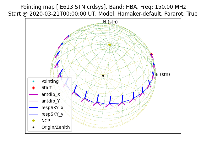
which shows a unit IAU X/Y component as it appears to station’s X/Y antennas as the source moves across the celestial sky (Note that a LOFAR station’s coord. sys. is not necessarily aligned with the celestial coord. sys.); and also this:
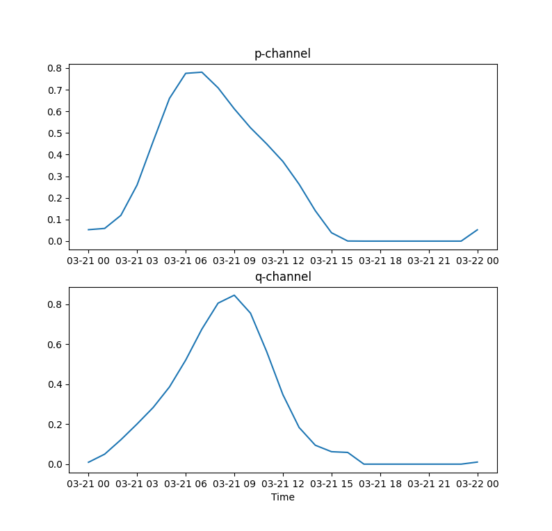
which shows the apparent source flux in the X/Y-channels (denoted ‘p/q’ here).
Querying telescope details
dreamBeam is designed to be used with any radio telescope by using a plugin
interface. To find out which telescopes pointing_jones knows about we just
query it by leaving the queried argument blank. So e.g., if one runs:
$ pointing_jones print
Specify telescope:
  NenuFAR, LOFAR
Usage:
  pointing_jones print|plot telescope band stnID beammodel beginUTC duration timeStep pointingRA pointingDEC [frequency]
You can see that the command responds with “Specify telescope:” and a list of selectable telescopes: “NenuFAR” and “LOFAR”. You can query other possible argument values in an analogous way (for band etc).
| [1] | This pulsar is a.k.a. LGM-1 or “Little Green Men”, which would be highly appropriate on this particular day :-) |